Perceptron in General

Introduction

We are going to take a better look at the starting point of machine learning and artificial neural network, the Perceptron. The creation of such algorithmic structure goes back to 1957 and was created by Frank Rosenblatt. Rosenblatt worked at Cornell Aeronautical Laboratory in Buffalo, New York, where he was successively a research psychologist, senior psychologist, and head of the cognitive systems section. Yes you heard it right machine learning techniques are far from being new. Rosenblatt demonstrated the use of his Perceptron by implementing it in a simulation running on a IBM 704 and then on a Mark 1. it was meant for image recognition purpose. The neuron was fed a series of punch cards. After 50 trials, the computer learned to distinguish cards marked on the left from cards marked on the right !

Biological neurons

The brain is maded of cells called neurones connected one to another and linked by synapses. Information is circulating in the form of electric signals in neurons, then in a chemical form at the synapse level. A given neuron receives informations coming from other neurons. If the cumulation of incoming signals is strong enough, it will send a signal itself. This phenomenon is called summation.

Perceptron an artificial neuron

Inputs and weights

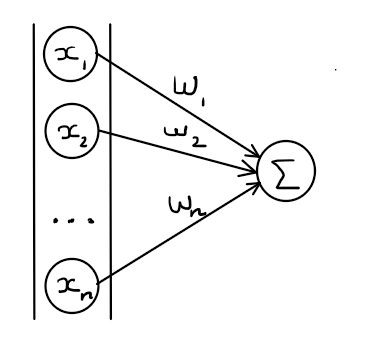
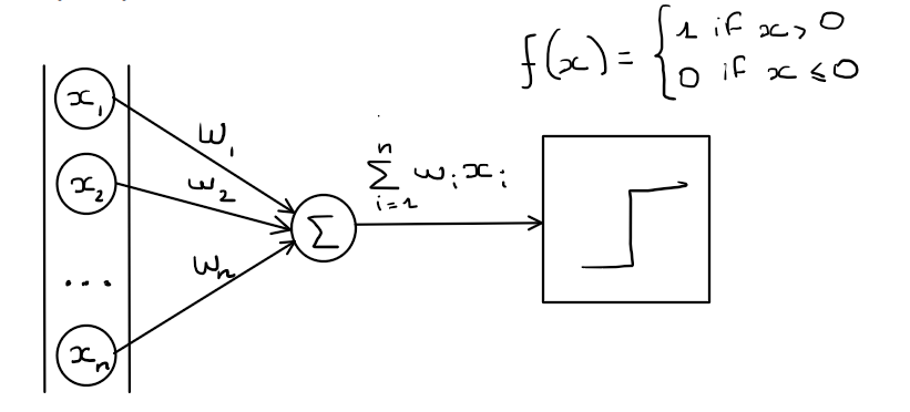
The Perceptron receives numbers $x_1, x_2, …,x_n$ as inputs. We can view those incoming numbers as signal coming from other neurons. Since connections are not equals, some links are stronger than other, between the input and the neuron, we need a way to mathematically represent this. To the input we are applying what is called weights $w_1, w_2, …,w_n$ each of those weights are associated to the given connection with the input. For simplicity let’s say that inputs and weights are numbers between $0$ and $1$, meaning that a strong connection is close to $1$ and a weak one close to $0$. Each signal coming toward the neurons is then said to be ${x_1w_1, x_2w_2,…,x_nw_n }$.

Summation

Now we need to calculate the cumulation of those incoming signals, this is the summation to be precise we are doing spatial summation. It is the algebraic summing of potentials from different areas of input, usually on the dendrites. In the above graph this is the unit containing the $\sum$ symbol that is responsible for this part of the process. This process is really simple we take the weighted sums of the inputs:

\[\sum_{i=1}^{n}w_ix_i\]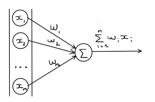

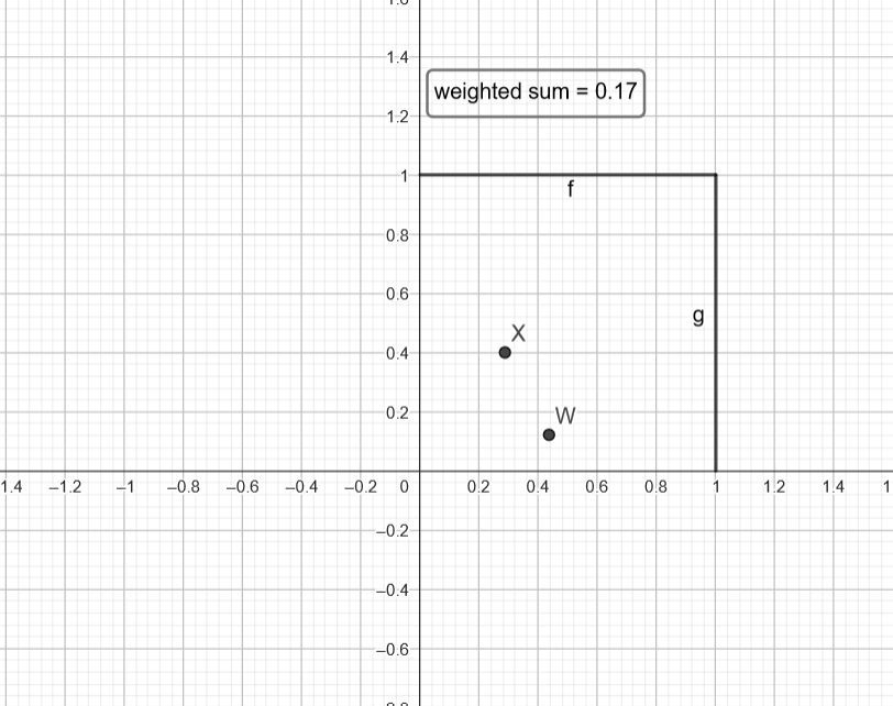
Where $X=(x_1,x_2)$ and $W=(w_1,w_2)$ for $X=(0.29,0.4)$ and $W=(0.44, 0.12)$ we get $weighted sum = 0.29\times0.44+0.4\times0.12=0.17$.

Activation function

We said that a neuron is fired if the sum of the incoming signals is strong enough, well what does it mean do be fired, and what is the threshold to make this event occur?

When we say a neuron is “fired,” it means that it generates an output signal, which then propagates through the network. This output signal is the neuron’s way of communicating with other neurons in the network.

The threshold to trigger the firing of a neuron is determined by the activation function applied to the sum of the incoming signals. The activation function is a mathematical function that introduces non-linearity into the neural network, allowing it to learn complex patterns and make decisions based on the input it receives.

The activation function takes the weighted sum of the inputs to the neuron, which includes the inputs from the previous layer (or the input layer in the case of the first layer) and the biases associated with each neuron. The activation function then applies a transformation to this sum, and if the result exceeds a certain threshold, the neuron is activated or ‘fired’. Otherwise, it remains inactive.

Different activation functions can be used in neural networks, each with its own characteristics and advantages. Some common activation functions include the step function, sigmoid function, hyperbolic tangent (tanh) function, and rectified linear unit (ReLU) function. These functions introduce non-linearity and allow the neural network to learn complex relationships and make more accurate predictions.

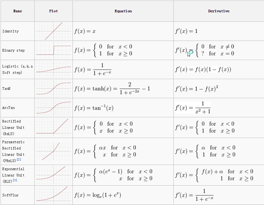
In our case we will choose the easiest one to understand, our Perceptron will either be fired which means an output of $1$ or unfired in this case $0$. To achieve these results we will be using the Binary step function :

\[θ(x) = \begin{cases} \text{0 for } x < 0\\ \text{1 for } x \geq 0 \end{cases}\]

Wait, you might ask how can we get a value such that $θ(x) = 0$ if $\sum_{i=1}^{n}w_ix_i >= 0$ since $x_i, w_i \in [0, 1]$ ? Well what about updating the binary step function so that it uses a threshold $T$ ? \(θ(x) = \begin{cases} \text{0 for } x < T\\ \text{1 for } x \geq T \end{cases}\)

Normally it is not a problem we could also not used a $T$ and kept with 0 but since in our case we have specified our weights to be in $[0,1]$, they will not be updated outside those bonds during the learning process. Don’t worry, it is only to introduce a new idea called bias. Normally we don’t set bounds for the Perceptron parameters.

Bias

The bias term plays a crucial role in the functioning of a perceptron. The bias allows for more flexibility in decision-making by introducing an additional parameter that can shift the activation function’s decision boundary.

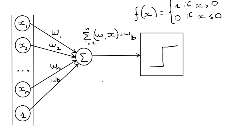
The bias term, denoted as $b$, is a learnable parameter associated with each neuron in a neural network, including the perceptron. It serves as an offset or bias, adjusting the activation of the neuron. Mathematically, the weighted sum of inputs ($\sum_{i=1}^{n}w_ix_i$) is modified by adding the bias term, resulting in $\sum_{i=1}^{n}w_ix_i + b$.

By incorporating the bias term, we can control the decision boundary of the perceptron. The bias acts as an additional input with a fixed value of 1. It is associated with a weight parameter ($w_b$), which determines the impact of the bias on the output.

The bias allows the perceptron to fire or activate even when all the input values are zero. It essentially adjusts the threshold at which the perceptron will be fired. If the weighted sum of inputs, along with the bias term, is greater than or equal to zero, the perceptron will be fired (output 1); otherwise, it will remain inactive (output 0).

We will visualise this introduced bias as a input and weight combination, such as $x_b=1$ and $w_b = b$, where $b$ is our threshold.

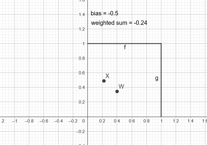
And voila, even with inputs and weights (excluding the bias one) strictly positive we get a negative weighted sum, using this shifting process.

Output

Now how the neuron can be fired from our example we said fired is $1$ and not fired is $0$. But it does not have to be this way, we saw that a lot of activation functions exist and some of them display interesting behavior. Where the step function has only two possible states, the other activation functions can produce a wider range of output values. This allows for more nuanced and continuous activation levels rather than a simple binary decision.

For example, the sigmoid function is a popular choice for activation in neural networks. It has a characteristic S-shaped curve and maps the input to a value between 0 and 1. The sigmoid function is defined as:

\[σ(x)=\frac{1}{1+e^{-x}}\]

Here, $e$ is the base of the natural logarithm. The sigmoid function assigns higher activation levels to inputs that are positive and closer to 1, while inputs that are negative and closer to 0 are assigned lower activation levels. The sigmoid function allows for a smooth transition between these two extremes, providing a continuous output range.

Activation functions like sigmoid are beneficial in scenarios where the magnitude and relative strength of activation are important. They can capture more nuanced patterns in the data by assigning different levels of activation to different input values.

In contrast, the binary step function has a limited range and provides a simple binary decision. While it can still be useful in certain cases, the use of activation functions with a wider range of outputs allows neural networks to perform more complex computations and make finer distinctions in the output predictions.

But what those output numbers represent? Remember the Perceptron goals is to make binary classification, the goal is that given a set of data points the Percepetron can say that such point is a part of class A and the other are part of a class B.

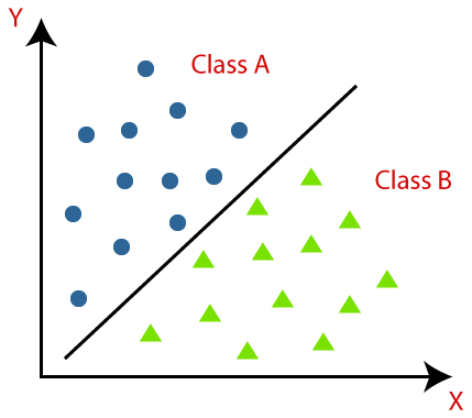
One important fact is that the points need to be linearly separable for the Perceptron to work, this means that for points of both class, we can draw a line between points from class A and class B. If we go on a higher dimension, we need a hyperplan separating the classes.

We call this ‘line’ the decision boundary.The decision boundary is determined by the weights and biases of the perceptron. It represents the specific combination of input values that will result in a change in the perceptron’s output classification.

We will see how to visualise it, but first we need to know how the Perceptron learns.

Learning process

The learning process of a perceptron involves iteratively adjusting its weights and biases to find the optimal values that allow it to accurately classify the given data points. This process is known as training the perceptron.

It is a supervised learning algorithm, we need our data points to be labeled either A or B and then we see how the Perceptron classifies each points, in our case, if the output is 0 let’s say it is classified as being A, and if 1 the point is classified as B.

The goal of the training process is to slap the perceptron and telling him he’s wrong when misclassifying points, when this occurs he needs to update his weights based on the received feedback.

Here’s the algorithm for training :

• Initialization : Initialize the weight values ($w_i$) and the bias ($w_b$) of the perceptron.
• Forward Propagation :For each data point in the training dataset, calculate the weighted sum of the inputs ($\sum_{i=1}^{n}w_ix_i$) and apply the activation function to produce the output prediction ($\hat{y}$).
• Error Calculation : Compare the predicted output $\hat{y}$ to the true label $y$ of the data point to calculate the prediction error.
• Backpropagation : Adjust the weights and bias based on the error. The weight updates are calculated by multiplying the error by the input values and the learning rate ($\alpha$), and adding the result to the current weights. The bias update is equal to the error multiplied by the learning rate.
• Repeat : Repeat steps 2 to 4 for all data points in the training dataset.

You see that I’ve introduced a new notion above, the learning rate $\alpha$, this is a hyperparameter of our algorithm, which means that the learning rate is not learned from the data but set manually before training the perceptron. The learning rate controls the step size of weight updates during the learning process.

Choosing an appropriate learning rate is crucial for the convergence and performance of the perceptron. If the learning rate is too large, the weight updates can be too drastic, causing the perceptron to overshoot the optimal solution and potentially diverge. On the other hand, if the learning rate is too small, the training process may be slow, and the perceptron may take a long time to converge.

Forget about the fact that in previous example we set a boundary of $[0, 1]$.

For our example let’s take 2 points of class A and B:

• $A = (0.1, 0.5)$
• $B = (0.5, 0.1)$

And set the following parameters for our Peceptron :

• $w = (0.5, 0.5)$
• $b = 0$, remember we can view it as a weight $w_b$ linked to an input of $1$.
• $\alpha$ = 1
• Activation function : Binary Step Function

Now let’s run the algorithm :

• Forward Propagation :

  A :

  Weighted sum: $0.5 \times 0.1 + 0.5 \times 0.5 + 0 = 0.3$ Activation: $θ(0.3) = 1$ (since $0.3 \geq 0$)

  B :

  Weighted sum: $0.5 \times 0.5 + 0.5 \times 0.1 + 0 = 0.3$ Activation: $θ(0.3) = 1$ (since $0.3 \geq 0$)

• Error Calculation :

  A :

  True label: Class A (expected output: 1) Predicted output: 1 Error: 0 (Correct classification)

  B :

  True label: Class B (expected output: 0) Predicted output: 1 Error: 1 (Misclassification)

• Backpropagation :

  Since there was a misclassification for Point B, we need to update the weights and bias.

  B :

  Update weight vector: $w_{new} = w + \alpha \times \text{error} \times \text{input} = (0.5, 0.5) + (1 - 0) \times 1 \times (0.5, 0.1) = (1, 0.6)$

  Update bias: $b_{new} = b + \alpha \times \text{error} = 0 + 1 \times 1 = 1$

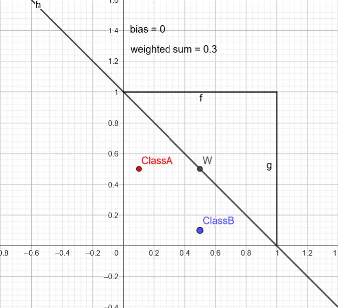
Now we continue the process until the classification is good. Let’s see exactly what is happening, on the graph the decision boundary is already drawn, I will explain how it is calculated in this case. But first let’s redo each step.

After checking each point we get a weighted sum of 3 in both case, but B is misclassified !

After enough steps we might converge in the following way. Note : I’ve cheated using geogebra and tweaking the weights and bias value to get this result.

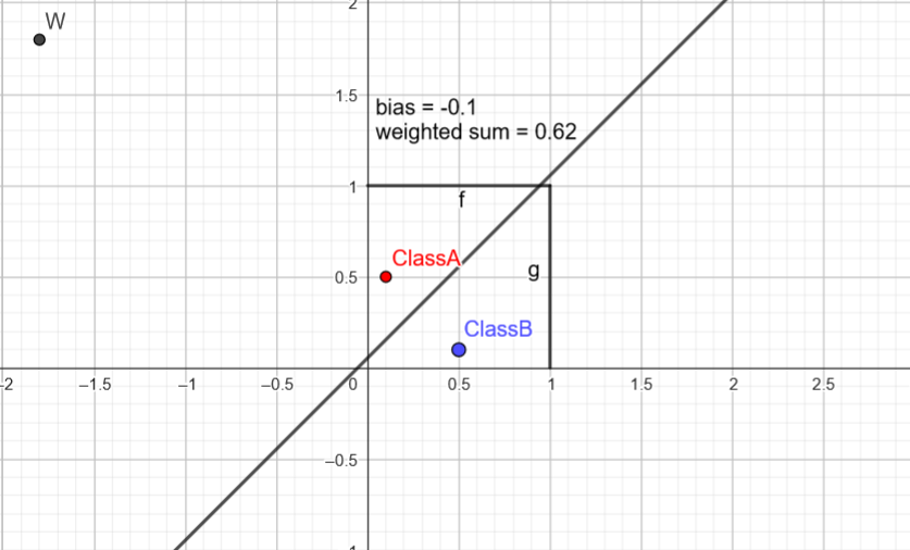
With this configuration the bounding boundary separate in 2 parts the points, the classification is achieved! How did we calculate the boundary for visualization?

Well, the idea is to check where point would be labelled as both A and B, we search this limit, equivalent to solving the following equation:

\(w1​⋅x1​+w2​⋅x2​+b=0 \text{, where } x_2 \text{ is the y absis.}\) This can be rewritten as : \(y = \frac{-b -w_1 * x}{w_2} = -\frac{w_1}{w_2}x-\frac{b}{w_2}\) And that’s our decision boundary in the the 2d space, in a higher dimensional space the idea remains the same but we are talking about hyperplane.

Conclusion

We saw the overall inner working of the building block of Artificial Neural Network, the Perceptron. t’s important to note that the perceptron is a foundational concept, and more complex neural network architectures have been developed to handle more intricate tasks. Nevertheless, understanding the perceptron provides a solid foundation for comprehending artificial neural networks and their applications.

In a future post, we will see how to implement a Perceptron class in Python and visualize the learning process steps.